Statistical Analysis of Performance Data Part 1 - Averages
Published on 27 Jun 2011Tags #Average #EdgeSight #Excel #Performance #Standard Deviation #Statistics
In the first article about the statistical analysis of performance data, I will be dealing with averages. I will explain why it is a bad idea to work with averages of averages (like when storing intermediate results), why relying on averages can be dangerous and what good averages look like.
For a full list of articles published in this series, please refer to the primer.
Intermediate Results
Performance analysis usually generates huge amounts of data. This often forces us to aggregate data by storing averages over a certain time interval instead of the individual values. Although this seems to be a very convenient way of saving space and time, you need to be extremely careful when processing those aggregated values because – in general – you are not allowed to calculate the average of average values.
Only in a very special situation are you allowed to proceed in this manner: When you are working with averages that are calculated from the exact same number of values, you receive a mathematically correct result. Have a look at the proof at the end of the article.
Fortunately, there is an easy remedy to this problem. By retaining the sum and the number of the values you are on the mathematically save side and you are able to aggregate your data to save space and time. This is why Citrix EdgeSight stores at least two values per metric (like processor_time_sum and processor_time_cnt in vw_system_perf).
Downside of Using Averages
It is often considered sufficient to judge a series of values by the average value. Unfortunately, the average is susceptible to outliers. Consider the following series of values: 10, 10, 10, 10, 10, 10, 10, 10, 10, 0. The average over all values is 9 but the set contains an outlier (value 0). By excluding the outlier the average rises to 10. Apparently, the initial average has been off by 10%.
It is especially problematic to use averages when the data set includes sequences of very low or even no values. This is often the case when considering server load over time. If a server is only used during business hours (e.g. between 7am and 7pm) only half the values can be considered to be useful values. Twelve hours of low or even no load will have an especially dramatic effect on the average load. This may cause peak usage to be disguised by seemingly normal load indicators. Ultimately, users will be complaining about slow response times.
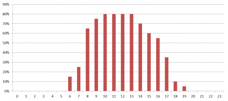
The following chart displays hourly load values for a single server over a single day. Apparently, the average load per day will be wrong by a large percentage due to the hours with low load:
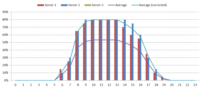
Therefore it is necessary to exclude nightly hours by filtering for business hours. When considering average values for a whole server farm, some servers may be configured to not take part in load balancing and therefore not accept user sessions. This causes average values to be much lower.
The effect of wrongly including zero values can easily be analyzed in a spreadsheet. Most spreadsheet applications provide a function for calculating the average value from a column of values, like AVERAGE in Microsoft Excel. This may not lead to the desired outcome. Instead a slightly more complex formula removes apparent outliers: SUMIF/COUNTIF or even easier AVERAGEIF. See this Excel file for a demonstration of these functions.
Although your spreadsheet application offers similar functions, you need to be very careful about considering values to be outliers. From a mathematical point of view you either need to have very good arguments for excluding values or need to use a well-known method to ensure a statistically correct result. I will expand on this topic in a later article of this series.
Recognizing “Good” Averages
The easiest way to recognize good average values is to be skeptical. Always take a close look at the minimum and maximum values to get a first impression about how far the values are spread.
Some months ago, I analyzed a series of latency values. The average value was far too high and kept me wondering how users were able to work at all. A closer look at the data set revealed incorrect values that must have been caused by an error in the product because it reported negative latency values and several impossibly high values in the billions. I decided to exclude those values as they were obviously caused by a software error.
There are several properties of a series of values that can hint towards a trustful average. The standard deviation is a common value to judge how far the values are spread around the average. A small standard deviation (when compared to the average) shows the values to be clustered around the average. But your data set may contain very high as well as very low values. In which case, the standard deviation correctly reports a very widely spread data set. I will present an approach to analyzing such a data set in a later article of this series.
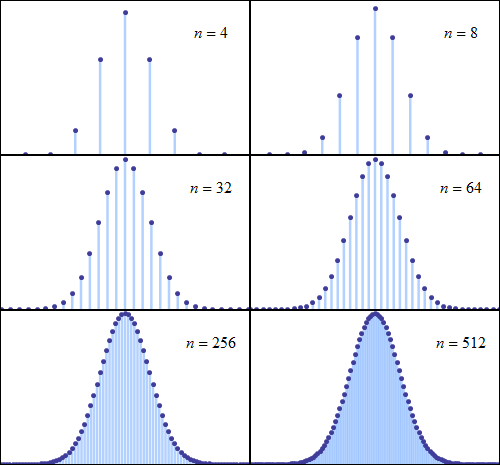
Many statistical properties of a data set assume that you are analyzing normally distributed values (see image below) which many data sets indeed are. Usually the peak value is set off to the left or right and the peak may be higher or lower. Just because your values do not look like they are distributed similarly to such a curve usually only means that you do not have a sufficiently high number of values.
(Source: Wikipedia about Normal distribution, image http://en.wikipedia.org/wiki/File:De_moivre-laplace.gif)
For such a normally distributed data set, the average value is equal to the mean. To determine the mean value, you need to sort your data set in ascending order and select the value that has an equal number of values on the left and on the right side. This property of a normal distribution leads to the insight that an average is more trustful when it is close to the mean of the data set.
Working with Few Values
Another downside of statistical analysis is the case of looking at a small data set. When your data set consists of less than 30 values, many statistical properties may not provide a secured insight.
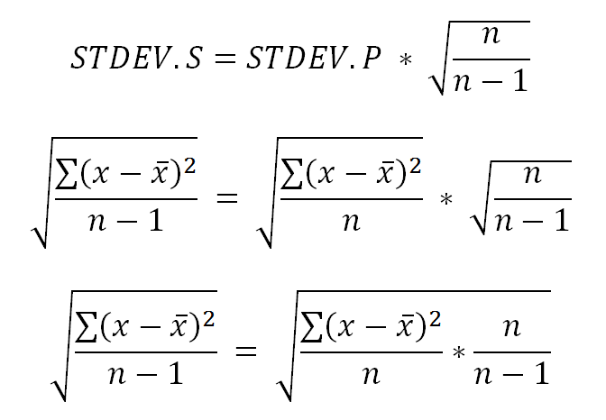
For example, the standard deviation needs to be corrected by a small factor based on the number of values. Microsoft Excel offers two functions for calculating the standard deviation, STDEV.S and STDEV.P. The latter assumes that your data set has a sufficient number of values whereas STDEV.P is calculated from STDEV.S by multiplying by SQRT(N/(N-1)) with N being the number of values. See the end of this article for the mathematical connection between these two functions.
Fortunately, in performance analysis you are usually confronted with too many values. Although this may cause other problems (like the maximum number of rows in Excel 2003), from a statistical point of view this is a very comfortable situation!
Mathematical Proof: Why is the Average of an Average a Dangerous Thing?
This section contains the mathematical proof why calculating the average of averages is only valid in a very special case. I will reduce the problem to the average of two averages.
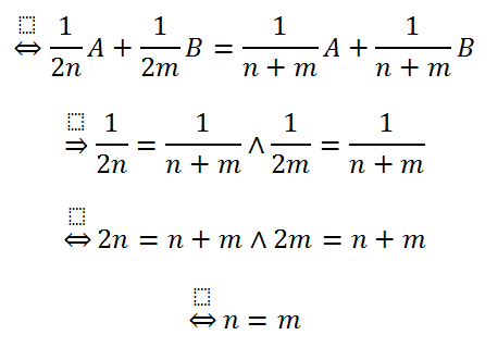
Let’s consider the following two sets of values. The first set consist of values a1, …, an and the second set consist of values b1, …, bm. The left side of the first line represents the average of the two averages and the right side shows the average over all the individual values.
To make the equation more readable, I have substituted the sums with upper letters, so that A represents the sum of all ai and B represents the sum of all bj.
The remaining lines are basic algebraic operations to simplify the equation.
Apparently, the initial equation is only valid if n and m are the same value. This translates to the result that the average of averages may only be used when the individual data sets have exactly the same size.
Mathematical Connection between both Functions for Calculating the Standard Deviation
Excel offers two functions for calculating the standard deviation. STDEV.P assumes that your data represents the entire population – meaning that you have all the data there is. Therefore, this function is only suited for large data sets with 30 or more values. During performance analysis, this is the only function to be used because we usually have more than enough values.
In case, you have less than 30 values, you must either use STDEV.S or apply a correction to STDEV.P as displayed below.
Apparently, the right-hand side can be simplified to be equal to the left-hand side.
